Basic introduction to Bayesian Methodology
Bayesian Methodology
Bayesian way of thinking
You have a belief that probability of getting a head(let’s say 0.8) is more than the tail because of your past experience. You challenge your friend in a long coin flipping contest for a period of 12 months. After every month, you update your previous belief based on new evidence of the coin flip and hence readjust the probability. After the end of the year, your belief of getting a head is 0.5 with some uncertainity involved.
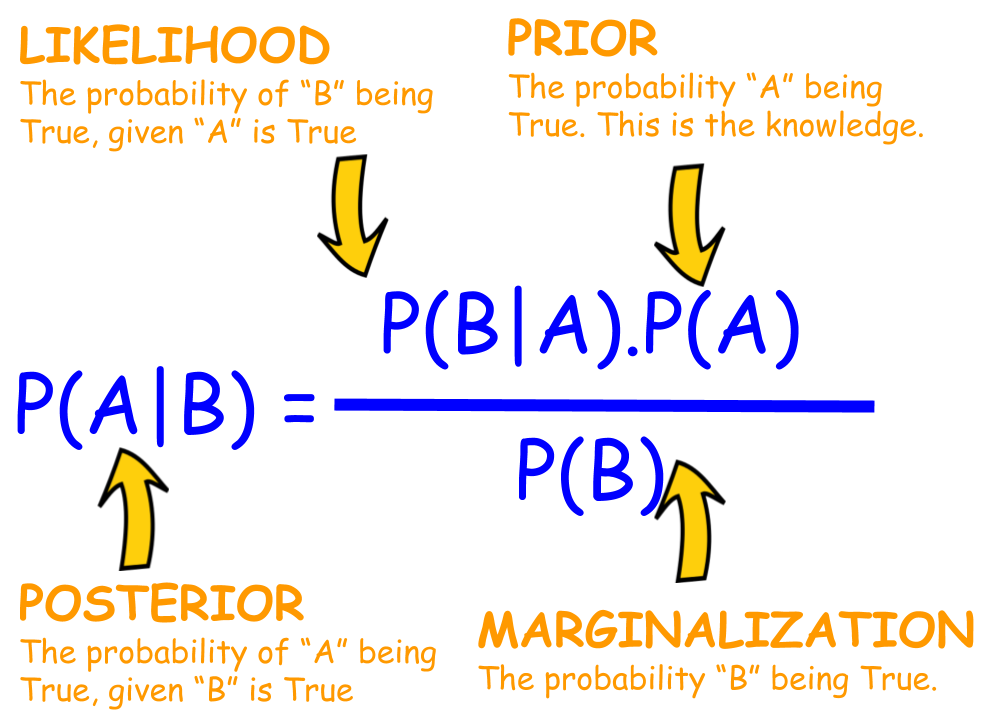
- In essence, Bayesian methodology is about having a prior belief (prior probability) of an event and updating that belief on seeing new evidence (likelihood) and hence as a result forming new belief (posterior probability) about the event.
Advantages of using a Bayesian approach
-
Bayes’s theorem helps in quantifying the uncertainity of an event using probabilistic model which differentiates it from the frequentist approach where a point estimate is calculated which doesn’t give much insight about the event.
-
Bayesian approach also integrates the domain knowledge(prior) of the event that we are modeling, thereby, providing a informative starting point for our model. Though, also note that an uninformative prior can be created to reflect a balance among outcomes when no information is available.
Random variable
-
A random variable is described as a variable whose values depend on a random process.
- For example, in the case of our coin flip challenge a variable
Xcould be considered as a random variable whose value could either be 1(head) or 0(tail) depending on the outcome of coin flip(random process) - Here
Xis a discrete random variable as it can only take discrete values. Discrete data can only take certain values, for example: number of students in a class, we can’t have half a student.

- Temperature, age, height, weight are all examples of continuous random variable as it can take infinitely many values. For example, a random variable measuring the time taken for something to be done is continuous since there are an infinite number of possible times that can be taken.
- For example, in the case of our coin flip challenge a variable
Probability Distribution
-
It can be considered as a function which takes in a random variable, let’s say
Xand assign probabilities to each of it’s outcome.- Bernoulli distribution can be used to represent the random variable
Xmodelling two possible outcomes. A bernoulli distribution is discrete, as opposed to continuous, since only 1 or 0 is a valid response.
- The most commonly used distribution is the Gaussian distribution,also referred as Normal distribution or bell curve is used frequently in finance, investing, science, and engineering.


-
It is so popular mainly because of three reasons:
- Ubiquitous in natural phenomena
- Incredible number of processes in nature and social sciences naturally follows the Gaussian distribution. Even when they don’t, the Gaussian gives the best model approximation for these processes.
- Mathematical Reason: Central Limit Theorem
- Central limit theorem states that when we add large number of independent random variables, irrespective of the original distribution of these variables, their normalized sum tends towards a Gaussian distribution. For example, the distribution of total distance covered in an random walk tends towards a Gaussian probability distribution.
- Once a Gaussian, always a Gaussian!
Unlike many other distribution that changes their nature on transformation, a Gaussian tends to remain a Gaussian.
- Product of two Gaussian is a Gaussian
- Sum of two independent Gaussian random variables is a Gaussian
- Convolution of Gaussian with another Gaussian is a Gaussian
- Fourier transform of Gaussian is a Gaussian
- Simplicity
- For every Gaussian model approximation, there may exist a complex multi-parameter distribution that gives better approximation. But still Gaussian is preferred because it makes the math a lot simpler!
- Its mean, median and mode are all same
- The entire distribution can be specified using just two parameters- mean and variance
- Bernoulli distribution can be used to represent the random variable
Mathematical representation of Bayes’s theorem is given by,
There are specific techniques that can be used to quantify the probability for multiple random variables, such as the
joint,marginal, andconditional probability. These techniques provide the basis for a probabilistic understanding of fitting a predictive model to data.
Joint Probability
The probability of two (or more) events is called the joint probability.
For example, the joint probability of event A and event B is written formally as: P(A and B)
The “and” or conjunction is denoted using the upside down capital “U” operator “^” or sometimes a comma “,”.
P(A ^ B), P(A, B), P(AB)
The joint probability for events A and B is calculated as the probability of event A given event B multiplied by the probability of event B.
This can be stated formally as follows: P(A and B) = P(A given B) * P(B)
-
The calculation of the joint probability is sometimes called the fundamental rule of probability or the “product rule” of probability or the “chain rule” of probability.
-
Here,
P(A given B)is the probability of event A given that event B has occurred, called the conditional probability, described below. -
The joint probability is symmetrical, meaning that
P(A and B)is the same asP(B and A). The calculation using the conditional probability is also symmetrical, for example:P(A and B) = P(A given B) * P(B) = P(B given A) * P(A)
Marginal Probability
Marginal probability is the probability of an event irrespective of the outcome of another variable.
-
The probability of the evidence P(B) can be calculated using the law of total probability. If
P(B)is a partition of the sample space, which is the set of all outcomes of an experiment, then, - When there are an infinite number of outcomes, it is necessary to integrate over all outcomes to calculate
P(B)using the law of total probability. -
Often,
P(B)is difficult to calculate as the calculation would involve sums or integrals that would be time-consuming to evaluate, so often only the product of the prior and likelihood is considered, since the evidence does not change in the same analysis. The posterior is proportional to this product: - The maximum a posteriori, which is the mode of the posterior and is often computed in Bayesian statistics using mathematical optimization methods, remains the same. The posterior can be approximated even without computing the exact value of
P(B)with methods such as Markov chain Monte Carlo or Variational inference Bayesian methods.


Conditional Probability
The probability of one event given the occurrence of another event is called the conditional probability.
-
Types of event:
-
Independent event: Each event is not affected by any other events.
For example: Tossing of a coin, each toss of a coin is a perfect isolated thing. What it did in the past will not affect the current toss.
-
Dependent event: They can be affected by previous events
For example: Marbles in a bag.
2 blue and 3 red marbles are in a bag. What are the chances of getting a blue marble? The chance is 2 in 5, but after taking one out the chances change!
So the next time:
-
If we got a red marble before, then the chance of a blue marble next is 2 in 4
-
If we got a blue marble before, then the chance of a blue marble next is 1 in 4

-
-
P(B|A) is also called the “Conditional Probability” of B given A.
And in our case: P(B|A) = 1/4
So the probability of getting 2 blue marbles is:

And we write it as:

Probability of event A and event B equals the probability of event A times the probability of event B given event A.
Using Algebra we can also “change the subject” of the formula, like this:
Start with:
  P(A and B) = P(A) x P(B|A)
Swap sides:
  P(A) x P(B|A) = P(A and B)
Divide by P(A):
  P(B|A) = P(A and B) / P(A)
And we have another useful formula:
The probability of event B given event A equals the probability of event A and event B divided by the probability of event A.
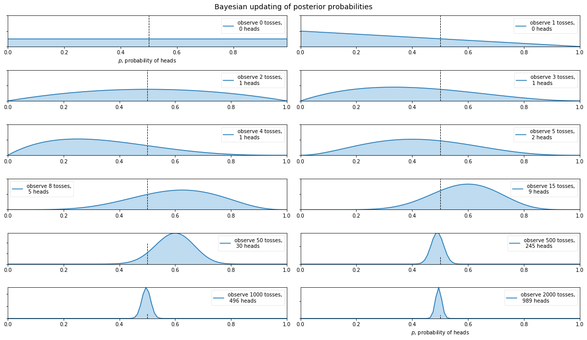
Coin flip example
View Code
%matplotlib inline
import scipy.stats as stats
import numpy as np
from matplotlib import pyplot as plt
from IPython.core.pylabtools import figsize

import tensorflow as tf
import tensorflow_probability as tfp
import collections

tfd = tfp.distributions

# tensorflow eager: tf ops immediately evaluated
# and produced as result

try:
  tf.compat.v1.enable_eager_execution()
except ValueError:
  pass

class _TFColor(object):
    """Enum of colors used in TF docs."""
    red = '#F15854'
    blue = '#5DA5DA'
    orange = '#FAA43A'
    green = '#60BD68'
    pink = '#F17CB0'
    brown = '#B2912F'
    purple = '#B276B2'
    yellow = '#DECF3F'
    gray = '#4D4D4D'
    def __getitem__(self, i):
        return [
            self.red,
            self.orange,
            self.green,
            self.blue,
            self.pink,
            self.brown,
            self.purple,
            self.yellow,
            self.gray,
        ][i % 9]
TFColor = _TFColor()


# Build Graph

rv_coin_flip_prior = tfd.Bernoulli(probs=0.5, dtype=tf.int32)

num_trials = tf.constant([0,1, 2, 3, 4, 5, 8, 15, 50, 500, 1000, 2000])

coin_flip_data = rv_coin_flip_prior.sample(num_trials[-1])

# prepend a 0 onto tally of heads and tails, for zeroth flip

coin_flip_data = tf.pad(coin_flip_data,tf.constant([[1, 0,]]),"CONSTANT")

# compute cumulative headcounts from 0 to 2000 flips,
# and then grab them at each of num_trials intervals

cumulative_headcounts = tf.gather(tf.cumsum(coin_flip_data), num_trials)

rv_observed_heads = tfd.Beta(
    concentration1=tf.cast(1 + cumulative_headcounts, tf.float32),
    concentration0=tf.cast(1 + num_trials - cumulative_headcounts, tf.float32))

probs_of_heads = tf.linspace(start=0., stop=1., num=100, name="linspace")
observed_probs_heads = tf.transpose(rv_observed_heads.prob(probs_of_heads[:, tf.newaxis]))

def evaluate(tensors):
    """Evaluates Tensor or EagerTensor to Numpy `ndarray`s.
    Args:
    tensors: Object of `Tensor` or EagerTensor`s; can be `list`, `tuple`,
      `namedtuple` or combinations thereof.

    Returns:
      ndarrays: Object with same structure as `tensors` except with `Tensor` or
        `EagerTensor`s replaced by Numpy `ndarray`s.
    """
    if tf.executing_eagerly():
        return tf.contrib.framework.nest.pack_sequence_as(
            tensors,
            [t.numpy() if tf.contrib.framework.is_tensor(t) else t
             for t in tf.contrib.framework.nest.flatten(tensors)])
    return sess.run(tensors)


# Execute graph

[num_trials_,
probs_of_heads_,
observed_probs_heads_,
cumulative_headcounts_,
] = evaluate([
  num_trials,
  probs_of_heads,
  observed_probs_heads,
  cumulative_headcounts
])

# For the already prepared, I'm using Binomial's conj. prior.

plt.figure(figsize(16.0, 9.0))
for i in range(len(num_trials_)):
    sx = plt.subplot(len(num_trials_)/2, 2, i+1)
    plt.xlabel("$p$, probability of heads") \
    if i in [0, len(num_trials_)-1] else None
    plt.setp(sx.get_yticklabels(), visible=False)
    plt.plot(probs_of_heads_, observed_probs_heads_[i],
             label="observe %d tosses,\n %d heads" % (num_trials_[i], cumulative_headcounts_[i]))
    plt.fill_between(probs_of_heads_, 0, observed_probs_heads_[i],
                     color=TFColor[3], alpha=0.4)
    plt.vlines(0.5, 0, 4, color="k", linestyles="--", lw=1)
    leg = plt.legend()
    leg.get_frame().set_alpha(0.4)
    plt.autoscale(tight=True)


plt.suptitle("Bayesian updating of posterior probabilities", y=1.02,
             fontsize=14)
plt.tight_layout()
This was originally written in a jupyter notebook which can be accessed here.